ICS4U – Machine Learning in Python
ICS4U Learning Goals
In this ICS4U Grade 12 Computer Science lesson you will be learning about
- Supervised vs Unsupervised vs Reinforcement Learning
- Creating a Model for a data set using a Machine Learning Algorithm
Types of Machine Learning
Machine learning is a subfield of AI that uses algorithms to make predictive models of various scenarios using data. Basically different algorithms have been designed to take large amounts of historical data, identify patterns in that data, and then come up with predictions for future data.
Some simple examples of this might be:
- Predicting Future Sales Values
- Making a Recommendation System for your favorite videos
- Classifying an image
- Supervised Learning
- Unsupervised Learning
- Reinforcement Learning
Predictive Models Using Linear Regression
You have been asked throughout high school to make predictive models in your Science and Math Classes. You might have been asked in science class to do an experiment where you changed the value of one variable (the independent variable) and recorded what happened to another variable. (the dependent variable), or you might be trying to analyze a correlation between two situations
For example:
- How is the stopping distance for a car affected by how fast it was going?
- How many goals will be scored by a hockey player based on the number of shots they take
- How much profit you will make based on how much you spend on social media advertising and tv advertising.
In order to analyze that data, you might have been asked to do the following:
- Graph the Data
- Draw a line of Best Fit Through the data
- Calculate the Slope of the Line of Best Fit
- Determine the Y intercept of the Line of Best Fit
- Create an equation y = mx+ b using that information
That y = mx + b equation is a predictive model, since you can now predict the y value based on a particular x value. This type of modelling is called Regression in Mathematics.
In this course we will stick with Two Variable Data because you can easily visual the data using a graph (1 independent variable and 1 dependent variable)
If the relationship between the variables is Linear, then this is called Linear Regression. If the data isn’t linear, its called Non Linear Regression.
Linear Regression Example
Situation:
- We have a set of data that relates 1 independent variable to 1 dependent variable
- The relationship between those variables is linear
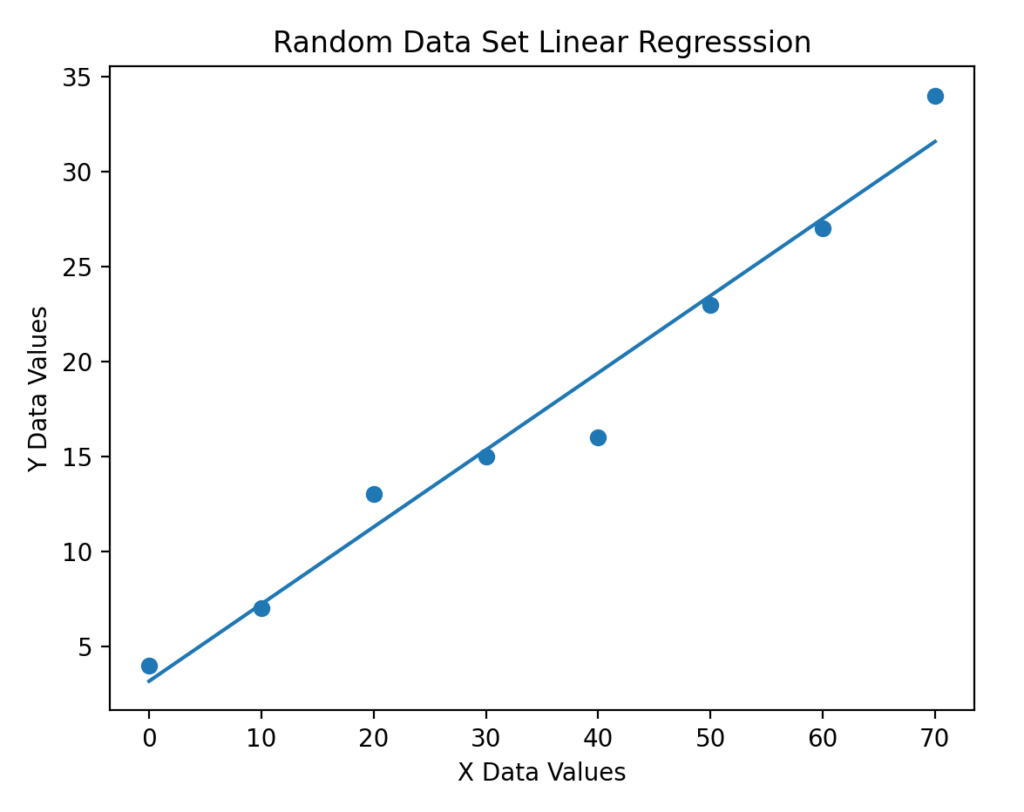
					#Example Data Set
x = [0,10,20,30,40,50,60,70]
y = [4,7,13,15,16,23,27,34]
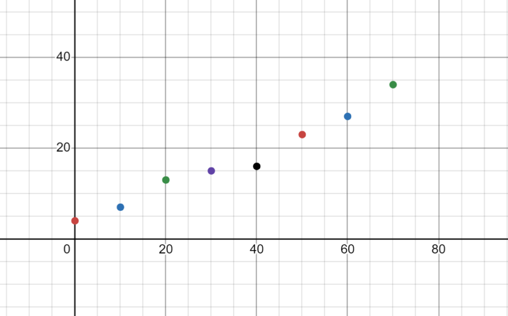
Goal:
- Make a predictive model in the form y = mx + b where you find the optimal values for the slope and the y intercept that keeps the line of best fit as close to all of the data points as possible
- Use the model to make predictions
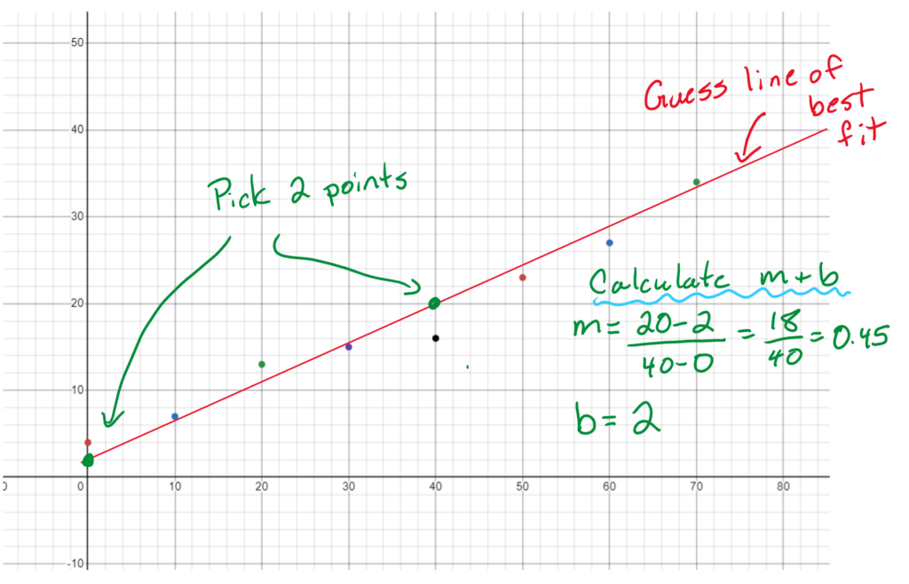
Option #1 - Guess
In Science class or in grade 9 math you were asked to basically just guess the line of best fit and use it to calculate the slope and y intercept. Not the most optimal solution, but it can work effectively.
- Draw your best guess of the line of best fit.
- Pick two points on the line of best fit and calculate the slope using rise/run
- Estimate the y intercept by looking at the graph.
Option #2 - Use a formula
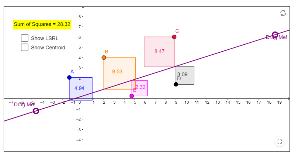
If you took Data Management (MDM4U) you were introduced to a formula that lets you calculate those values. It uses a method called least squares to find the minimum “error” between the points and the line of best fit.
- The vertical distance between the line of best fit and each data point is calculated (this is called a residual)
- Residuals are positive for points above the line, and negative for points below the line.
- For the optimal line of best fit, you want the sum of these residuals to be zero because then the line will be equal distance above some points and below some points.
- Least squares uses the squares of the residuals instead of the actual residuals themselves. The sum of the squares of the residuals needs to be the minimal possible value.
If you want to see how least squares regression works, then check out the following interactive website that lets you manipulate the data points and the line of best fit to visualize results
There is a formula that can be developed with calculus by using derivatives to find the line that minimizes the sum of the squares of the residuals.
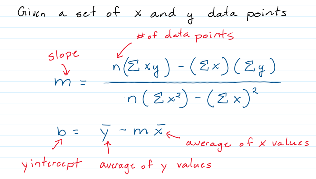
The Formula is easy to implement using what you have learned so far in python.
#Example Data Set
x = [0,10,20,30,40,50,60,70]
y = [4,7,13,15,16,23,27,34]
# Number of data points
n = len(x)
#Find Sum(x*y), Sum(x), Sum(y), Sum(x^2)
sumXY = 0
sumX = 0
sumXSq = 0
sumY = 0
for i in range(0,n):
sumXY = sumXY + x[i]*y[i]
sumX = sumX + x[i]
sumXSq = sumXSq + x[i] ** 2
sumY = sumY + y[i]
#Find average (mean) of x and y
meanX = sumX/n
meanY = sumY/n
#Find the slope
m = (n*sumXY - sumX*sumY)/(n*sumXSq - sumX**2)
#Find the y intercept
b = meanY - m * meanX
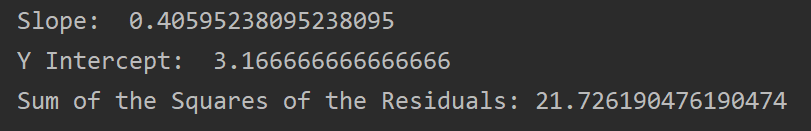
#Display the results
print("Slope: ", m)
print("Y Intercept", b)
Here is the data plot with the line of best fit, and the sum of the residual values.
Option #3 - Use Machine Learning
None of the above solutions used machine learning. But we we can also develop an algorithm where our code will “learn” the best value for the slope and y intercept using an algorithm called Gradient Descent
There is some different terminology and symbols that are used with machine learning algorithms that you should be familiar with. The terms slope and y intercept aren’t used. They are referenced as weights. The line of best fit formula is called the hypothesis function.
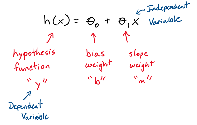
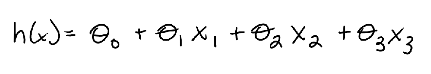
If there were more than 1 independent variable, then the hypothesis function would look like this. Each of x values represents a different independent variable affecting the dependent variable, and each theta represents how much influence that value has on the dependent variable. Higher theta = more influence
The goal is to minimize the difference between the y values of the hypothesis function and the y values of our data points. We will again be using the least squares approach. But this time we are going to use mean – squared – error That is just the average error across all the data points. In machine learning this error is often called the cost function
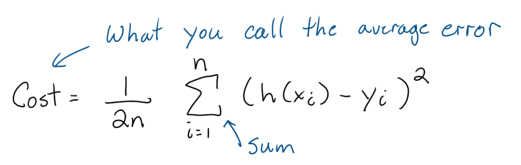
You will notice that there is an extra 2 in the denominator of this equation. You wouldn’t expect that to be there because to find an average you just divide by the number of data points. But there is a good reason why we add it to this formula. The goal is going to be to minimize this cost as the algorithm learns better values for the weights. This is done by taking derivatives. (Think calculus if you are taking it and optimization problems) That 2 in the denominator will cancel the 2 when taking the derivative of a square. So it just makes the math neater later on.
Gradient Descent
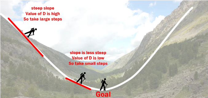
The process to minimize the cost function is called “Gradient Descent”. This is where the “learning” part of the algorithm comes into effect.
- The function to minimize is a quadratic that opens up. So it has a minimum value.
- When we are far away from the minimum the slope is steep. so we take big steps to get to the bottom.
- When the slope is shallow we take smaller steps to get closer to the minimum as not to overshoot.
FYI “Gradient” is another math term for Slope, often used in the international community.
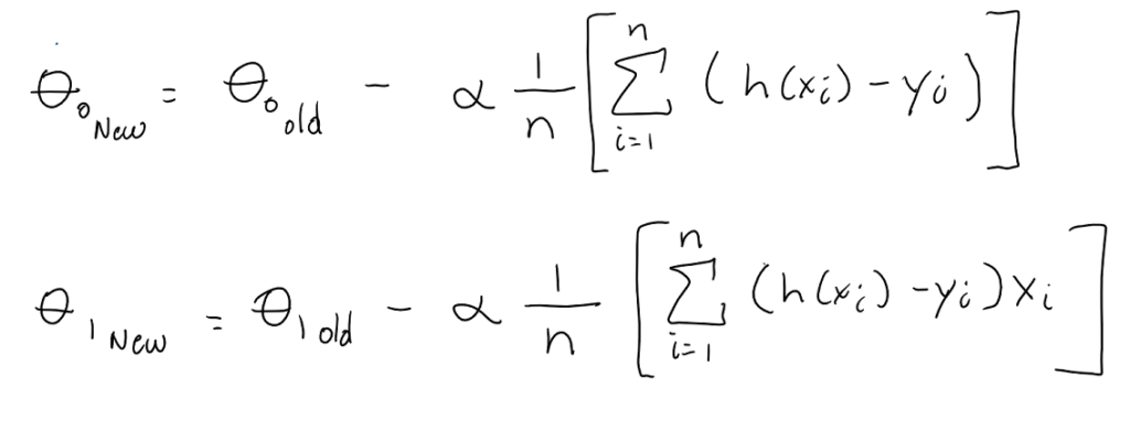
The next part is a little over your grade level mathematically, but it involves taking the derivative of the cost function with respect to each weight value and then predicting a new weight value based on those calculations.
You will notice another variable (alpha) has been added to the equations. This is called the learning rate. It is typically a really small value that controls how quickly we end up getting an answer. If its too small, then gradient descent just takes too long to get to the answer, and if its too big there is a chance that we overshoot the miniminum as you proceed down the curve.
You can keep calculating new weights over and over and over again, and in theory, the cost decreases every time that happens and your weight values get closer and closer to the optimal value. You would just have to decide how many iterations of the algorithm is appropriate. You might find the cost isn’t decreasing very much after a 1000 iterations, so its likely you are close to the true minimum and have an acceptable set of weights to complete the formula.
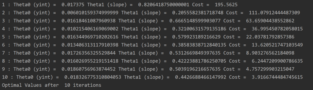
Here is the python implementation of the gradient descent algorithm. In the example there is a variable that controls the # of iterations. (iterations are often called epochs)
					#Number of iterations to do the gradient descent
epochs = 10

#Data Points you want to find the line of best fit for
x = [0, 10, 20, 30, 40, 50, 60, 70]
y = [4, 7, 13, 15, 16, 23, 27, 34]

#Initial Guess for weights
theta0 = 0  #y intercept
theta1 = 0  #slope

#learning rate
alpha = 0.001

#Number of Test Data points (x and y lists have to have same number of entries)
n = len(y)

#Perform the gradient descent
for e in range(0,epochs):

    #Calculate the cost using current theta values
    total = 0
    for i in range(0,n):
        total = total + (theta0 + theta1*x[i] - y[i])**2
    cost = 1/(2*n)*total

    #Learn New theta0
    total = 0
    for i in range(0,n):
        total = total + (theta0 + theta1*x[i] - y[i])
    theta0 = theta0 - alpha/n*total

    #Learn New theta1
    total = 0
    for i in range(0, n):
        total = total + (theta0 + theta1 * x[i] - y[i])*x[i]
    theta1 = theta1 - alpha / n * total


print("Optimal Values after ",epochs, "iterations")
print("Theta0 (yint) = ", theta0, "Theta1 (slope) = ", theta1, "Cost = ", cost)
Now I don’t have to calculate the cost every iteration, I’m just doing that so you can see how its changing after each iteration. You can see below that after 10 iterations, the cost is reducing as it should be.
The question becomes what is the optimal amount of iterations? There isn’t an exact answer, but here are some print outs of optimal values after different values of epochs.
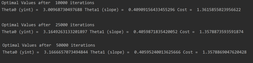
There isn’t really a change in values from 25000 to 50000 iterations, so its probably not worth running more then that. The cost (error) is also very low at this point as well. You need to decide what precision you want from the weights based on the application and how much computing power you have.
Alternative approaches to Gradient Descent:
- Normally machine learning is done with much more data then the example I showed you. Using regular lists is terribly inefficient in python with large data sets.
- Often a library called numpy is used instead. Numpy is optimized and has many useful math functions to accomplish these tasks using matrices and linear algebra (beyond the scope of this course)
- There is also a machine learning library for python called, Scikit-learn which can accomplish this task for us as well.
ICS4U Interactive Learning Activity - Grade 12 Computer Science
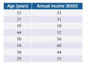
The following table shows salary levels for different aged employees at a small company. Write a program that allows the user to enter the age of an employee and have it output the predicted salary for that employee. Use the gradient descent algorithm in your solution.
Bonus if you can figure out MATPLOTLIB and make the plot so you can visualize the results
Classification Model - KNN
The K Nearest Neighbors algorithm is a simple machine learning algorithm that helps classify objects into a particular class (type). Its based on the assumption that similar types of object are found near to one another.
When doing a classification problem, you will have a data set that contains labels and classes
- The class is the type of objects that can be classified.
- The labels are the characteristics that define how to determine the class
For example, let’s say you were trying to classify a patient as being Diabetic or Not Diabetic. Some factors that influence diabetes are Age, Body Mass Index (BMI), glucose (sugar) levels.
- The data would probably be organized in some type of 2D list:
- Each row representing [Age, BMI, Glucose, Type]
- The Age, BMI, Glucose values would be the labels (inputs to the function)
- The Type would be the class (Diabetic / Not Diabetic) (outputs of the function)
Calculating Distance
There are several different ways to calculate “distance” to the nearest neighbors. Let’s use the one you would be familiar with from grade 10 math. That’s called Euclidian Distance. You are familiar with calculating the distance between 2 points on the Cartesian plan.
In that case you would be finding the distance from a Query point A to your input data point B. The data points in your Query Point and Your Input Data would have had 2 labels:
- One label representing the x coordinate
- One label representing the y coordinate
In General you would have a query point you are trying to classify, and a bunch of data points, and those data points could have any number of input labels.
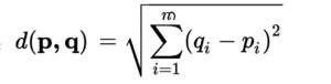
Here is the distance formula for a data point having m labels, with x as the data point, and q as the query point
Classifying the Data
This formula would be applied to every data point in the input set. So when that’s all done, you would have a list of distances from the query point to every data point in the input list.
You then pick the K closest input points to your query value and from that list see which class has the majority. That is pretty straightforward to accomplish as you could
- Sort the list in ascending order of distance
- Pick the first K values from that list
- Find the mode of the class types in the nearest neighbor list
The mode would represent the most likely choice for the class of your query data point.
Choosing K
There isn’t a sure fire way to decide what value of K is the best. It really depends on your data set. You don’t want it to be too small. You also don’t want it to be too big. Some trial and error is often necessary.
An Example:
Let’s say I want to classify an object based on its location in the 2D Plane. I have 2 types of objects. Red objects and Blue Objects.
Here is a visual of their locations.
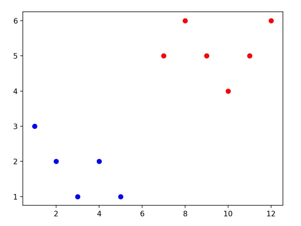
My goal is to take the location of a Query Point, and have my program predict if that object is a Red Object or a Blue Object.
I decided to take the data points and organize them into a 2 Dimensional list organized as follows: [xPosition , yPosition , Color]
					#Data Set with labels and classes
data = [
            [12,6,"R"],
            [7,5,"R"],
            [1,3,"B"],
            [8,6,"R"],
            [3,1,"B"],
            [10,4,"R"],
            [11,5,"R"],
            [4,2,"B"],
            [9,5,"R"],
            [2,2,"B"],
            [5,1,"B"]
]
The input for my program will simply be the x and y coordinates of a data point I wish to try an classify
					#The Query Point
query = [6,1]
Then I find the distances from that query point to all the data points in the input set
					import math

#Number of Data Points
n = len(data)

#Number of labels
m = len(data[0])-1

#A list to represent the distances
distances = []

#Find distance from the Query Point to every data point
for i in range(0,n):

    #For every label in the data set
    d = 0
    for j in range(0,m):
        x = data[i][j]
        q = query[j]
        d = d + (q-x)**2

    #Append the distance and class of the current data point
    cl = data[i][m]
    distances.append([math.sqrt(d),cl])
After this code is completed, the list distances will have the distance from the query point to each individual input point along with the type of object at that distance
For this example, I decided to use a K value of 3. So I’m going to sort the list in ascending order and pick the first 3 class values from that list. I don’t require the distances anymore, only the class types of the nearest neighbors.
					#Get the class values of the k nearest neighbors
k = 3
classList = []
distances.sort()
for i in range(0,k):
    classList.append(distances[i][1])
The only thing left now is to find the mode of the classList. I decided to use a function from the Counter Class in python to implement this.
					#Find the most common class of the k nearest neighbors
from collections import Counter
nn = Counter(classList)
classification = nn.most_common(1)[0][0]

#Output results
print("The object at postion (",query[0],",",query[1],") is classified as ",classification)
In the above example, the query point of (6,1) was classified as “B”
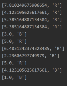
Here is a visual display of several query data points They show up as an X in the visualization, classified to the correct color.
ICS4U Interactive Learning Activity - Grade 12 Computer Science
Make sure you can get the algorithm above working on your machine
Bonus if you can figure out how to use MATPLOTLIB to create the data plot I used in the example
Non Linear Regression Model - KNN
The K Nearest Neighbors algorithm can be really easily adjusted to make a regression model.
During classification, the class is categorical (It’s a type of object) and you choose the most frequent class generated from your nearest neighbor list.
However, if you have a set of data, and you have a numerical class, you can predict the value of the class by calculating the average of the nearest neighbor list instead of the mode.
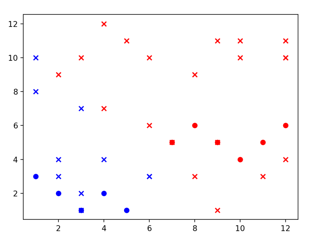
An Example
Suppose I wanted to make a predictive model of the following data set. In this case, the data list would have 1 label column (the x value of the data points) and 1 class column (the y value of the data points)
The query point would just be the x value that I would want to make a prediction for. If I wanted to predict the y value when x is -1 then I would set my query as follows.
					#The Query Point
query = [-1]
Then I find the distances from that query point to all the data points in the input set
					import math

#Number of Data Points
n = len(data)

#Number of labels
m = len(data[0])-1

#A list to represent the distances
distances = []

#Find distance from the Query Point to every data point
for i in range(0,n):

    #For every label in the data set
    d = 0
    for j in range(0,m):
        x = data[i][j]
        q = query[j]
        d = d + (q-x)**2

    #Append the distance and class of the current data point
    cl = data[i][m]
    distances.append([math.sqrt(d),cl])
For this example, I decided to use a K value of 3 again. So I’m going to sort the list in ascending order and pick the first 3 class values from that list. I don’t require the distances anymore, only the class values of the nearest neighbors. (Remember, those would be numbers in this example)
					#Get the class values of the k nearest neighbors
k = 3
classList = []
distances.sort()
for i in range(0,k):
    classList.append(distances[i][1])
Now I just need to find the average of the values in the nearest neighbor list.
					#Find the average of the classList
    predicted = sum(classList)/k
    print("Nearest Neighbours: ",classList, "Point:(",query[0],",",predicted,")")
So In this example, our regression algorithm predicted a y values of 3.97 when an x value of -1 was used
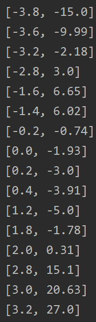
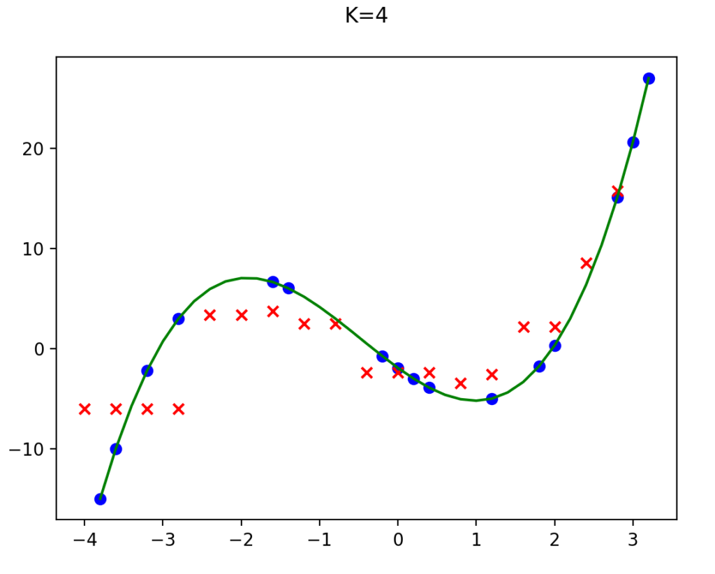
I ran the regression model with a bunch of data points and here is a visual display:
- Blue Dots are the training data set
- Green Line was the actual function I used to generate the data
- Red X points are the predictions of the model
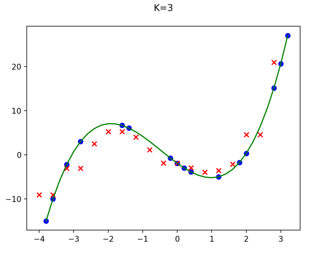
The model does well on the middle part of the function where there are more data points, but not so great near the edges. KNN would also have a problem extrapolating data outside of the training set because it would always be picking the same neighbors.
Out of curiosity, I ran the model with K values of 4 and 6 as well. Didn’t get as good of results.
One thing that is very different when comparing the linear regression model to the KNN model, is that with linear regression it produces a set of weights that you can use to make predictions. It only uses the training data once to get those weights, and then all predictions just use those weights and not the training data again. With KNN for every prediction it has to go through the entire training data set to find the nearest neighbors.
ICS4U Interactive Learning Activity - Grade 12 Computer Science
Make sure you can get the algorithm above working on your machine
- Have the training data read in from a comma delimited data file
- Instead of only having a single query value, make a list of query values to calculate. Predict all the values in the list and write them to a data file
Bonus if you can figure out how to use MATPLOTLIB to create the data plot I used in the example
Neural Networks
Neural Networks are a major part of Machine Learning. They are designed to mimic how the human brain works. They “learn” the rules from finding patterns in existing data sets. The idea has been around for a while, but only recently with additional computer power and the ability to run algorithms in parallel in modern GPU’s (Graphics cards) has the technology been made practical.
Using GPU's in Neural Networks
AI Learns To Play Tetris
Reinforcement Learning
Trying to figure out the math and coding behind reinforcement learning is probably beyond the scope of this course. But here are some videos I found interesting about the topic